Introduction to Predictions

Introduction

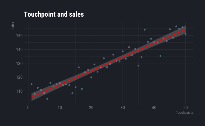
Suppose you are a sales manager in a company and you want to increase your sales. One of the possible ways could be to increase touch-points and/or sales manpower. You may want to find out what is the relationship between number of touch points and sales i.e. what will be the increase in sales if number of touch-points are increased by a specific amount. From our articles related to basics of data science, we know that scatterplot is one of the ways to visualize relationship between two numeric variables. The plot below shows one such plot.

library(ggplot2)
library(dplyr)

## 
## Attaching package: 'dplyr'

## The following objects are masked from 'package:stats':
## 
##     filter, lag

## The following objects are masked from 'package:base':
## 
##     intersect, setdiff, setequal, union

library(hrbrthemes)
import_roboto_condensed()

## You will likely need to install these fonts on your system as well.
## 
## You can find them in [/Library/Frameworks/R.framework/Versions/4.0/Resources/library/hrbrthemes/fonts/roboto-condensed]

set.seed(100)
data.frame(touchpoints=c(1:50),sales=c(100:149)+rnorm(50,mean = 5,sd=4)) %>% 
ggplot(aes(x=touchpoints, y=sales)) +
  geom_point() +
  stat_smooth(method="lm", colour="red") +
  labs(title = "Touchpoint and sales",
       x="Touchpoints",
       y="Sales") +
  theme_ft_rc()

## `geom_smooth()` using formula 'y ~ x'

Now, to understand how much will be the sales, given the number of touch points, one may assume that there is a linear relationship between the two i.e. 

$$

Sales = b(No. of Touchpoints)+c+

$$ b and c are some constants and epsilon is a random value. The red line shows the equation.

Now, it is not necessary that relationship will always be linear. It can be any function i.e.

\[ Y=f(X)+\epsilon \]

It is not necessary that there will be only one x. There can be several x or independent variables. When this function is unknown, we try estimate it. The different ways we try to estimate is what machine learning or statistical learning is. Lot of people will argue on what are the differences between statistical learning and machine learning. To put it simply, statistical learning models can be interpreted easily and hence very good at explaining the relationship between variables. Whereas, machine learning models can not always be interpreted. However, they tend to have higher accuracy. In words of Matthew Stewart, a PhD researcher from Harvard, Machine learning is all about results, it is like working in a company where your worth is characterized solely by your performance. Whereas statistical modeling is more about finding relationships between variables and the significance of those relationship, whilst also catering to prediction. However, there is no boundary to divide the two.

Hence the purpose of estimating the function f serves two purposes. One to predict the dependent variable y and to understand the relationship between x and y. This estimation of function f can be done in two ways. These are parametric and non-parametric models. In parametric models, a function is first assumed (like in the example of sales and touch-points, linear function was assumed). Then an attempt is made to estimate the coefficients. For example, if the assumed function is linear

\[ f(x)=\beta_0+\beta_1 \times x_1 + \beta_2 \times x_2 .... \beta_n \times x_n \]

Then we try to find out the values of the \(\beta s\) i.e we fit/train the model. The obvious attempt is create an equation that has least amount of difference from the original data points. THere are several ways to do it, which shall be discussed in due course.

Now, it is not easy to estimate or assume a function. If the assumption is far from reality, the estimates will be poor. To avoid such scenario, non-parametric methods can be used to estimate the function f. Here, instead of assuming a function and then trying to find the coefficients, the attempt is to find a suitable function. However, this approach require more parameters and large amount of data.

In general, there is a trade-off between interpretability and prediction accuracy. However, it is not always true. It is often observed that a more interepetable and less flexible model has better accuracy, because of overfitting.

Supervised and Unsupervised learning

Most of the machine learning or statistical learning problems fall under supervised or unsupervised learning. When you teach a child what a ball is by showing a ball and the child can then identify balls from a set of items, it is analogous to supervised learning. However, if you give a set of items to a child and ask her to segregate them, she may segregate them based on colour of the items i.e. all red coloured items in one group and all green coloured items in another. Or perhaps, she can identify other similarities. For example, some items with roofs are segregated in one category and some items with wheels are segregated in another. Here, how to identify the items was not taught to the child. Rather no instruction was given apart from asking her to segregate them. This is analogous to unsupervised learning. In our first example we had a specific prediction to make. We wanted to predict sales from number of touch-points. And to do that several data points were used that showed relationship between number of touch-points and sales. This is a classic example of supervised learning. We had supplied both dependent(y) and independent variable(x). In unsupervised learning we supply only independent variables (x) and the model calculates y based on different aspects. An example could be segmentation of customers. We can observe various characteristics of our customers (like spending pattern, age etc.) and then try to segment them.

Some of the problems may also fall under semi-supervised learning.

Classification and regression problems

Problems where response or outcome variable is quantitative are called regression problems. Problems where response or outcome variable are qualitative are called classification problems.

Measuring Accuracy

There is no one model that serves all problems. Each problem has a model that works best for the particular problem. The same model will not work for problems. This means, we need a way to understand and measure how good a model is.