Linear Regression
Linear regression is a very simple method of supervised learning. despite widespread use of advanced models it remains one of the most widely used method. In fact many advanced methods are extensions of linear methods. It is extremely important that a data scientist understands linear regression in all aspects.
Linear Regression
dt %>% knitr::kable()| District | Inhabitants | percent_below5k | percent_unemployed | Murder_pa_p1M | below5k | unemployed |
|---|---|---|---|---|---|---|
| 1 | 587000 | 16.5 | 6.2 | 11.2 | 96855 | 36394 |
| 2 | 643000 | 20.5 | 6.4 | 13.4 | 131815 | 41152 |
| 3 | 635000 | 26.3 | 9.3 | 40.7 | 167005 | 59055 |
| 4 | 692000 | 16.5 | 5.3 | 5.3 | 114180 | 36676 |
| 5 | 1248000 | 19.2 | 7.3 | 24.8 | 239616 | 91104 |
| 6 | 643000 | 16.5 | 5.9 | 12.7 | 106095 | 37937 |
| 7 | 1964000 | 20.2 | 6.4 | 20.9 | 396728 | 125696 |
| 8 | 1531000 | 21.3 | 7.6 | 35.7 | 326103 | 116356 |
| 9 | 713000 | 17.2 | 4.9 | 8.7 | 122636 | 34937 |
| 10 | 749000 | 14.3 | 6.4 | 9.6 | 107107 | 47936 |
| 11 | 7895000 | 18.1 | 6.0 | 14.5 | 1428995 | 473700 |
| 12 | 762000 | 23.1 | 7.4 | 26.9 | 176022 | 56388 |
| 13 | 2793000 | 19.1 | 5.8 | 15.7 | 533463 | 161994 |
| 14 | 741000 | 24.7 | 8.6 | 36.2 | 183027 | 63726 |
| 15 | 625000 | 18.6 | 6.5 | 18.1 | 116250 | 40625 |
| 16 | 854000 | 24.9 | 8.3 | 28.9 | 212646 | 70882 |
| 17 | 716000 | 17.9 | 6.7 | 14.9 | 128164 | 47972 |
| 18 | 921000 | 22.4 | 8.6 | 25.8 | 206304 | 79206 |
| 19 | 595000 | 20.2 | 8.4 | 21.7 | 120190 | 49980 |
| 20 | 3353000 | 16.9 | 6.7 | 25.7 | 566657 | 224651 |
We shall try to explain the method using an example. We have a data set where we have some information
- Population (Inhabitants) of different districts
- Number & percentage of people who earn below $ 5k pa out of the population
- Number & percentage of people unemployed and
- Murder rate per 1 M people, p.a.
Murder rate is the dependent variable. We want to know the following. 1. If there is a relationship between unemployment or income with murder rate? 2. If there is a relationship, how strong is it? 3. Do both unemployment and income effect murder rate? 4. How accurately can we predict the effect of unemployment/income on murder rate? 5. How accurately can we predict murder rate, given unemployment/income 6. Does unemployment and low income together has some additional effect on murder rate?
While using linear method, we assume that there is a linear relationship between the dependent and response variable. For example, we can assume that murder rate is linearly related with unemployment.
\[
\hat {MurderRate} \approx \hat \beta_0+ \hat \beta_1(unemployment)
\]
Please note that we are using an approximate sign and the betas and murder rate have hats on their head. This is because the function and the coefficients (betas) ar all estimates.
Now, we need to use the data points that we have (for example {6.2, 11.2}, {6.4, 13.4} ….) to estimate the values of the coefficients (betas) so that the linear model fits well. This mean, we want to find out the value of \(\beta_0\) and \(\beta_1\) which produces a line that is closest to all the 20 data points that we have. How close, can be calculated in several ways, of which least square is widely used.
Suppose we fit a line using a set of coefficients and predict the murder rate. The predicted value will be different from the real value. When these differences are squared and added up, it is called residual sum of squares. In this example
\[ RSS=({MurderRate}_{real}^{district1}-{MurderRate}_{predicted}^{district1})+..+({MurderRate}_{real}^{district20}-{MurderRate}_{predicted}^{district20}) \]
When we fit another line (Using another set of coefficients), we will get another RSS. And if we continue fitting new lines, we will keep on getting new RSSs. Least square helps us find the line (the coefficients \(\beta_0\) and \(\beta_1\)) that has the lowest RSS. To generalize it,
\[ RSS=e_1^2+e_2^2+e_3^2+....+e_n^2 \\ \implies RSS= (y_1-\hat y_1)^2 +(y_2-\hat y_2)^2 + .... + (y_n-\hat y_n)^2 \\ \implies RSS=(y_1-\hat \beta_0- \hat \beta_1x_1)^2 + (y_2-\hat \beta_0- \hat \beta_1x_2)^2 +...+ (y_n-\hat \beta_0- \hat \beta_1x_n)^2 \\ RSS = \sum_{i=1}^n(y_i-\hat\beta_0-\hat\beta_1x_i)^2 \]
Mathematicians and statisticians have already established the formula for \(\beta_0\) and \(\beta_1\) which minimizes RSS.
\[ \beta_0=\bar y- \beta_1 \bar x \]
and
\[ \beta_1= \frac{\sum_{i=1}^n(x_i-\bar x)(y_i - \bar y)}{\sum_{i=1}^n(x_i - \bar x)^2} \]
\(\bar x\) and \(\bar y\) are sample means.
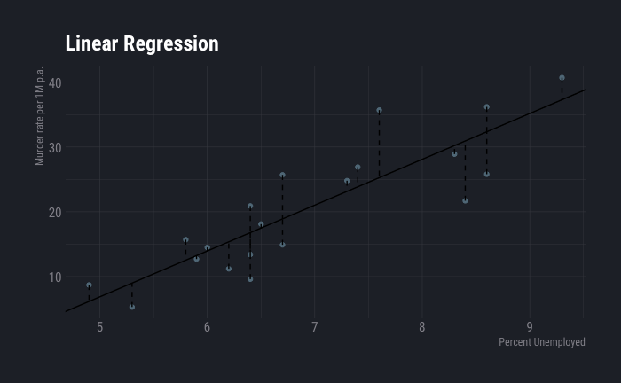
Let us apply linear method on the data we have using unemployment rate as independent variable.
dtlm <- lm(dt$Murder_pa_p1M ~ dt$percent_unemployed, data=dt)

dt$slope <- coef(dtlm)[2]
dt$intercept <- coef(dtlm)[1]
dt$y_hat <- (dt$slope * dt$percent_unemployed) + dt$intercept


dt %>%
  ggplot( aes(x=percent_unemployed, y=Murder_pa_p1M)) +
  geom_point() +
  geom_abline(aes(slope=slope,intercept=intercept),show.legend=F) +
  geom_segment(aes(x=percent_unemployed,y=Murder_pa_p1M,xend=percent_unemployed,yend=y_hat),show.legend=F, linetype=2) +
  labs(
    title ="Linear Regression",
    y="Murder rate per 1M p.a.",
    x="Percent Unemployed"
  ) +
  theme_ft_rc()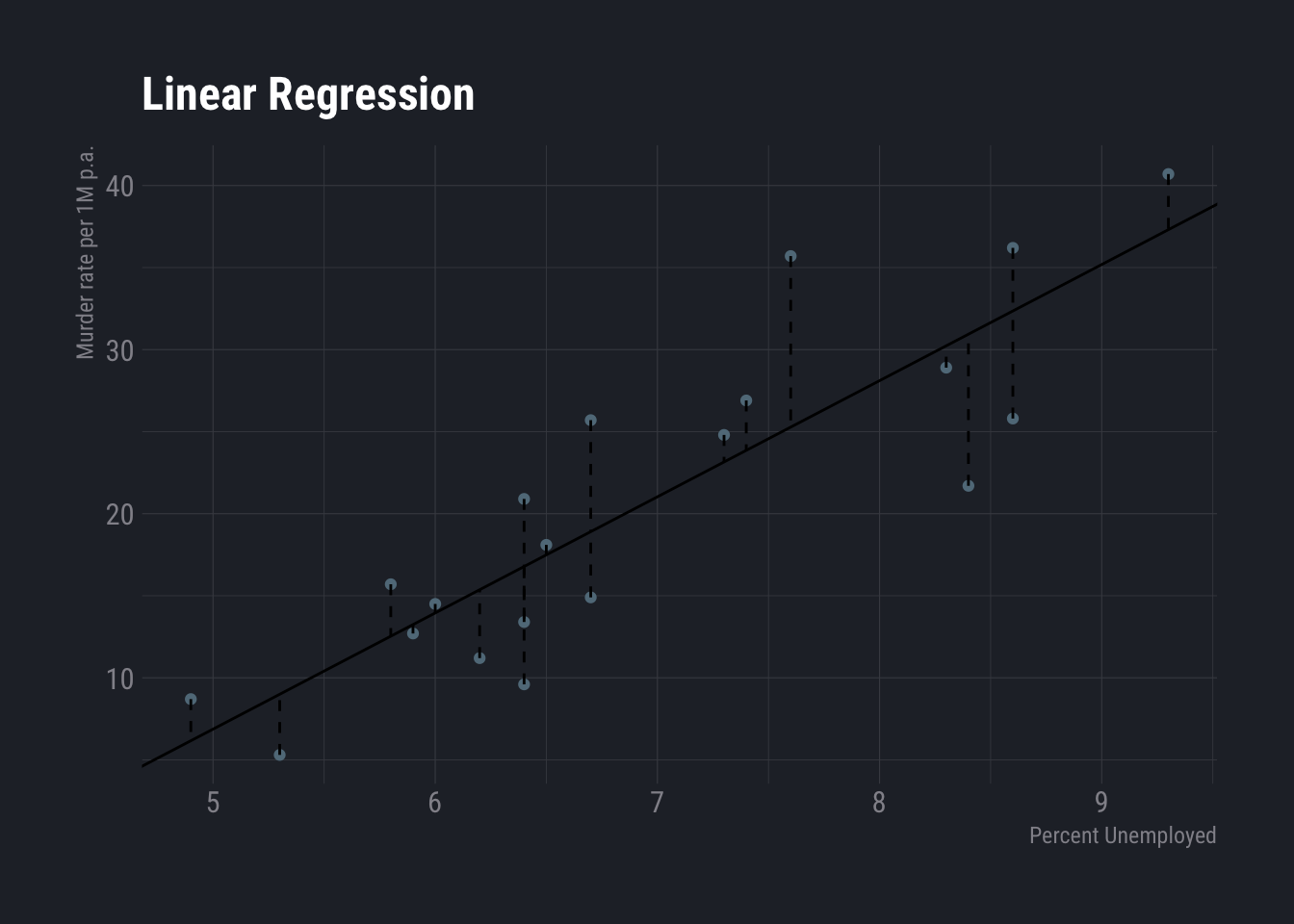
Here \(\beta_0\) is -28.5267089 and \(\beta_1\) is NA. According to this, each percent increase in unemployment increases murder rate by around 7 units.
Our estimation of \(\beta_0\) and \(\beta_1\) are based on sample data. These values for the population may be different. TO understand how much is the difference, we will use the concepts of standard error. Standard errors for the coefficients are given by
\[ SE(\hat \beta_0)^2= \sigma^2[\frac{1}{n}+\frac{\bar x^2}{\sum_{i=1}^n(x_i-\bar x^2)}] \\ SE(\beta_1^2)=\frac{\sigma^2}{\sum_{i=1}^n(x_i-\bar x)^2} \] $ ^2$ is the variance of \(\epsilon\), the errors or difference between predicted values and real values. $ $ is known as residual standard error
\[ RSE= \sqrt{RSS/(n-2)} \]
The standard errors are used to calculate the confidence intervals. S0, 95 % confidence interval for $ _x $ is
\[ \beta \pm 2 . SE(\beta) \]
From our example, following are the confidence intervals
confint(dtlm)## 2.5 % 97.5 %
## (Intercept) -42.841799 -14.211619
## dt$percent_unemployed 5.044454 9.114655Intercept is $ _0 $. So, we can conclude with 95 % confidence that change in each percent of unemployment rate can increase the unemployment rate by 5.04 to 9.11 units.
summary(dtlm)##
## Call:
## lm(formula = dt$Murder_pa_p1M ~ dt$percent_unemployed, data = dt)
##
## Residuals:
## Min 1Q Median 3Q Max
## -9.2415 -3.7728 0.5795 3.2207 10.4221
##
## Coefficients:
## Estimate Std. Error t value Pr(>|t|)
## (Intercept) -28.5267 6.8137 -4.187 0.000554 ***
## dt$percent_unemployed 7.0796 0.9687 7.309 8.66e-07 ***
## ---
## Signif. codes: 0 '***' 0.001 '**' 0.01 '*' 0.05 '.' 0.1 ' ' 1
##
## Residual standard error: 5.097 on 18 degrees of freedom
## Multiple R-squared: 0.748, Adjusted R-squared: 0.7339
## F-statistic: 53.41 on 1 and 18 DF, p-value: 8.663e-07Whether the independent value has some influence on the dependent variable is obtained from the p value. If p value is very small, we can conclude that the influence of the independent variable on the response variable is significant. To understand how accurate the model is, Residual standard error is often used. However, this, being in the units of y, may be confusing. A better way is to use R-squared, which describes the proportion of variance of the errors explained by the model. It is always between 0 and 1. A higher value indicates large proportion of the variance has been explained by the model and generally, the model is strong. If the value is low, then the assumed linear relation is invalid and/or the inherent error is high.
We can follow similar logic if we want to include multiple parameters.
dtlm <- lm(Murder_pa_p1M ~ percent_unemployed+percent_below5k, data=dt)
summary(dtlm)
##
## Call:
## lm(formula = Murder_pa_p1M ~ percent_unemployed + percent_below5k,
## data = dt)
##
## Residuals:
## Min 1Q Median 3Q Max
## -5.9019 -2.8101 0.1569 1.7788 10.2709
##
## Coefficients:
## Estimate Std. Error t value Pr(>|t|)
## (Intercept) -34.0725 6.7265 -5.065 9.56e-05 ***
## percent_unemployed 4.3989 1.5262 2.882 0.0103 *
## percent_below5k 1.2239 0.5682 2.154 0.0459 *
## ---
## Signif. codes: 0 '***' 0.001 '**' 0.01 '*' 0.05 '.' 0.1 ' ' 1
##
## Residual standard error: 4.648 on 17 degrees of freedom
## Multiple R-squared: 0.802, Adjusted R-squared: 0.7787
## F-statistic: 34.43 on 2 and 17 DF, p-value: 1.051e-06Please note that, to understand if at least one of the variables have influence on the independent variable, it is always better to use the F-statistic measure or the corresponding p-value. This is because, there is still 5 % chance that a variable appears to be significant just by chance.
Once it is established that at least one of the variable has influence on the response variable, the next step is to identify which variables are important or more important than others. To identify that, p-values (Pr(>|t|)) are used again. However, as mentioned in last paragraph, it is possible that some of the lower p-values occur just by chance. One way to overcome this problem is to try out different models. For example, if there are 2 independent variables, one can consider four models. 1. One with no variable (Null model) 2. One with both the variables and 3. Two models each with one of the two variables.
Suppose we have these four models. How do we select the best out of these? There are some statistics that help us do it, like AIC and BIC etc. We will cover these later. Now, modeling all possible models may be very hectic. If p is the number of independent variables, there are $ 2^p $ possible models. If there are 25 variables, this number becomes 3.355443210^{7}. Fitting this many models is not prudent. To solve this problem, three possible approaches can be used.
- Forward Selection: In this we start with a Null model. Then we fit a linear model with all variables and the variable with lowest p-value is added to the null model. This is continued till a certain objective is achieved.
- Backward Selection: In this we start with all the variables and remove the one with highest p-value. The we fit the model again to remove the variable with highest p-value. We repeat this till our object is reached.
- Mixed: In this model, we start with the forward selection approach. However, in the process, if it is observed that p-value of one of the variable has exceeded some threshold, it is removed.
We spoke about statistics like AIC and BIC. One may ask, why not use the R-squared? One of the reason is that when we add more variables, automatically R-squared increases even if by a small amount.
summary(lm(Murder_pa_p1M ~ percent_unemployed+percent_below5k+below5k, data=dt))##
## Call:
## lm(formula = Murder_pa_p1M ~ percent_unemployed + percent_below5k +
## below5k, data = dt)
##
## Residuals:
## Min 1Q Median 3Q Max
## -5.7220 -3.3108 0.3889 1.7897 9.9360
##
## Coefficients:
## Estimate Std. Error t value Pr(>|t|)
## (Intercept) -3.619e+01 6.872e+00 -5.266 7.68e-05 ***
## percent_unemployed 4.744e+00 1.534e+00 3.092 0.00699 **
## percent_below5k 1.151e+00 5.643e-01 2.040 0.05816 .
## below5k 4.227e-06 3.524e-06 1.200 0.24777
## ---
## Signif. codes: 0 '***' 0.001 '**' 0.01 '*' 0.05 '.' 0.1 ' ' 1
##
## Residual standard error: 4.59 on 16 degrees of freedom
## Multiple R-squared: 0.8183, Adjusted R-squared: 0.7843
## F-statistic: 24.02 on 3 and 16 DF, p-value: 3.627e-06In the model above, I added the variable below5k which is the absolute number of people in the district with income below 5k. Now, using this and the variable percent_below5k are in a way redundant and adds no value. Despite this, the R-squared has increased slightly. We should be aware of this and avoid reliance on slight increase in R-squared. You may also observe the slight decrease in RSE.
When we predict using a model, there are two kinds of errors - reducible and irreducible. Reducible is the one which can be reduced by different methods including tweaking of the model. And irreducible ones are much like random noise and we do not have the knowledge or the tools yet to reduce it. When we spoke about confidence interval, it covers only the later. To cover both the errors, prediction interval is used.
Below we are predicting a value with prediction interval.
dtlm <- lm(Murder_pa_p1M ~ percent_unemployed+percent_below5k, data=dt)

predict(dtlm, newdata = data.frame(percent_unemployed=10,percent_below5k=7), interval = "predict")
## fit lwr upr
## 1 18.48434 -7.522375 44.49105And predicting again with confidence interval.
predict(dtlm, newdata = data.frame(percent_unemployed=10,percent_below5k=7), interval = "confidence")## fit lwr upr
## 1 18.48434 -5.60224 42.57092You may notice that prediction interval is wider than confidence interval. Prediction interval is used when predicting single value. While predicting large number of values, confidence interval is used. For example, if unemployment rate and percent of low-income population are a and b for n number of districts, what is the average murder rate of those districts. Here we use confidence interval. But if we want to predict the murder rate in a district where unemployment rate and percent of low-income population are a and b, we use prediction intervals.
One may ask how does we include qualitative variables in the model. It is not that one will have only quantitative variables in the observed data. Well, dummy variables are created to translate qualitative variables into new set of quantitative variables. So, if you have a qualitative variable where there are two different values (for example gender, male and female), you can create a variable and mark one as 1 and other as 0. If there are more than two values (say gender, male, female, gender-neutral) then you can create two new variables. Say male and female and mark them as 1 or 0 according to your nomenclature to identify the gender. R automatically takes care of this. So, you do not need to create the variables yourself.
Non linear. Or not?
Till now we have used the following on our example data.
\[ Y=\beta_0+\beta_1X_1+\beta_2X_2+\epsilon \] In this model, we are missing out the possible additional effect of two variables occurring together. This is called interaction of variables. In our example, perhaps, occurrence of unemployment and low income together creates additional effect. We can use the following model to capture that.
\[ Y=\beta_0+\beta_1X_1+\beta_2X_2+\beta_3 X_1 X_2 +\epsilon \] Let us try it on our example
dtlm <- lm(Murder_pa_p1M ~ percent_unemployed+percent_below5k+percent_unemployed*percent_below5k, data=dt)

summary(dtlm)
##
## Call:
## lm(formula = Murder_pa_p1M ~ percent_unemployed + percent_below5k +
## percent_unemployed * percent_below5k, data = dt)
##
## Residuals:
## Min 1Q Median 3Q Max
## -6.255 -2.842 0.296 1.886 9.915
##
## Coefficients:
## Estimate Std. Error t value Pr(>|t|)
## (Intercept) -51.1746 50.0560 -1.022 0.322
## percent_unemployed 6.7314 6.9408 0.970 0.347
## percent_below5k 2.0969 2.5972 0.807 0.431
## percent_unemployed:percent_below5k -0.1165 0.3378 -0.345 0.735
##
## Residual standard error: 4.774 on 16 degrees of freedom
## Multiple R-squared: 0.8035, Adjusted R-squared: 0.7666
## F-statistic: 21.8 on 3 and 16 DF, p-value: 6.753e-06Seems like in this case the interaction does not exist.
Going further, we can also include non-linear components. For example square or cube of a variable.
\[ Y=\beta_0+\beta_1X_1+\beta_2X_2^2+\epsilon \] Let us try applying this on our example
dtlm <- lm(Murder_pa_p1M ~ I(percent_unemployed^2)+percent_below5k, data=dt)

summary(dtlm)
##
## Call:
## lm(formula = Murder_pa_p1M ~ I(percent_unemployed^2) + percent_below5k,
## data = dt)
##
## Residuals:
## Min 1Q Median 3Q Max
## -5.7810 -2.5357 0.2352 1.3456 10.6976
##
## Coefficients:
## Estimate Std. Error t value Pr(>|t|)
## (Intercept) -18.6013 7.9695 -2.334 0.0321 *
## I(percent_unemployed^2) 0.2997 0.1129 2.655 0.0166 *
## percent_below5k 1.2344 0.6023 2.049 0.0562 .
## ---
## Signif. codes: 0 '***' 0.001 '**' 0.01 '*' 0.05 '.' 0.1 ' ' 1
##
## Residual standard error: 4.768 on 17 degrees of freedom
## Multiple R-squared: 0.7917, Adjusted R-squared: 0.7671
## F-statistic: 32.3 on 2 and 17 DF, p-value: 1.621e-06Again, in this example there is no value addition of adding the non-linear components. However, let me use another data set from R to show an example below.
mtcars## mpg cyl disp hp drat wt qsec vs am gear carb
## Mazda RX4 21.0 6 160.0 110 3.90 2.620 16.46 0 1 4 4
## Mazda RX4 Wag 21.0 6 160.0 110 3.90 2.875 17.02 0 1 4 4
## Datsun 710 22.8 4 108.0 93 3.85 2.320 18.61 1 1 4 1
## Hornet 4 Drive 21.4 6 258.0 110 3.08 3.215 19.44 1 0 3 1
## Hornet Sportabout 18.7 8 360.0 175 3.15 3.440 17.02 0 0 3 2
## Valiant 18.1 6 225.0 105 2.76 3.460 20.22 1 0 3 1
## Duster 360 14.3 8 360.0 245 3.21 3.570 15.84 0 0 3 4
## Merc 240D 24.4 4 146.7 62 3.69 3.190 20.00 1 0 4 2
## Merc 230 22.8 4 140.8 95 3.92 3.150 22.90 1 0 4 2
## Merc 280 19.2 6 167.6 123 3.92 3.440 18.30 1 0 4 4
## Merc 280C 17.8 6 167.6 123 3.92 3.440 18.90 1 0 4 4
## Merc 450SE 16.4 8 275.8 180 3.07 4.070 17.40 0 0 3 3
## Merc 450SL 17.3 8 275.8 180 3.07 3.730 17.60 0 0 3 3
## Merc 450SLC 15.2 8 275.8 180 3.07 3.780 18.00 0 0 3 3
## Cadillac Fleetwood 10.4 8 472.0 205 2.93 5.250 17.98 0 0 3 4
## Lincoln Continental 10.4 8 460.0 215 3.00 5.424 17.82 0 0 3 4
## Chrysler Imperial 14.7 8 440.0 230 3.23 5.345 17.42 0 0 3 4
## Fiat 128 32.4 4 78.7 66 4.08 2.200 19.47 1 1 4 1
## Honda Civic 30.4 4 75.7 52 4.93 1.615 18.52 1 1 4 2
## Toyota Corolla 33.9 4 71.1 65 4.22 1.835 19.90 1 1 4 1
## Toyota Corona 21.5 4 120.1 97 3.70 2.465 20.01 1 0 3 1
## Dodge Challenger 15.5 8 318.0 150 2.76 3.520 16.87 0 0 3 2
## AMC Javelin 15.2 8 304.0 150 3.15 3.435 17.30 0 0 3 2
## Camaro Z28 13.3 8 350.0 245 3.73 3.840 15.41 0 0 3 4
## Pontiac Firebird 19.2 8 400.0 175 3.08 3.845 17.05 0 0 3 2
## Fiat X1-9 27.3 4 79.0 66 4.08 1.935 18.90 1 1 4 1
## Porsche 914-2 26.0 4 120.3 91 4.43 2.140 16.70 0 1 5 2
## Lotus Europa 30.4 4 95.1 113 3.77 1.513 16.90 1 1 5 2
## Ford Pantera L 15.8 8 351.0 264 4.22 3.170 14.50 0 1 5 4
## Ferrari Dino 19.7 6 145.0 175 3.62 2.770 15.50 0 1 5 6
## Maserati Bora 15.0 8 301.0 335 3.54 3.570 14.60 0 1 5 8
## Volvo 142E 21.4 4 121.0 109 4.11 2.780 18.60 1 1 4 2dtlm<-lm(hp~disp+wt+I(qsec^2), data=mtcars)
summary(dtlm)##
## Call:
## lm(formula = hp ~ disp + wt + I(qsec^2), data = mtcars)
##
## Residuals:
## Min 1Q Median 3Q Max
## -38.231 -24.310 -2.222 11.369 112.553
##
## Coefficients:
## Estimate Std. Error t value Pr(>|t|)
## (Intercept) 207.9443 40.7046 5.109 2.06e-05 ***
## disp 0.1866 0.1338 1.394 0.17421
## wt 19.0971 15.5313 1.230 0.22908
## I(qsec^2) -0.5153 0.1189 -4.334 0.00017 ***
## ---
## Signif. codes: 0 '***' 0.001 '**' 0.01 '*' 0.05 '.' 0.1 ' ' 1
##
## Residual standard error: 33.74 on 28 degrees of freedom
## Multiple R-squared: 0.7813, Adjusted R-squared: 0.7579
## F-statistic: 33.35 on 3 and 28 DF, p-value: 2.212e-09Here, we have used the square of qsec.
Precautions with linear modeling
One needs to take care of certain things while or before using linear models. These are
- Check for outliers and high leverage points
- Check for collinearity or multicollinearity
- Non-constant variance of errors
- Non-linearity of data and
- Correlation of error terms
Outliers are points for which response variable is extremely high and high leverage points are points where independent variable value is extremely high. They interfere with RSE and r-squared and must be removed.
Collinearity is when independent variables are correlated. THey can usually be identified using correlation matrix. However, when multiple variables are correlated (multicollinearity), they are not easy to identify in correlation matrix. One can use variance inflation factor to identify those and keep only one of the correlated variables.
Non-constant variance in errors of heteroscedasticity can be observed from residual plot. When a residual plot forms a funnel like shape, i.e. narrow band in one end that gradually increases as you progress across the axis. When facing this problem, one can try transforming the response variable concave functions like log or square root.
dtlm <- lm(ncases~., data=esoph)
ggplot(dtlm, aes(x = .fitted, y = .resid)) +
  geom_point()+
    labs(
    title ="Residual Plot",
    subtitle = "Observed funnel or cone shape",
    y="Residuals",
    x="fitted Values"
  ) +
  theme_ft_rc()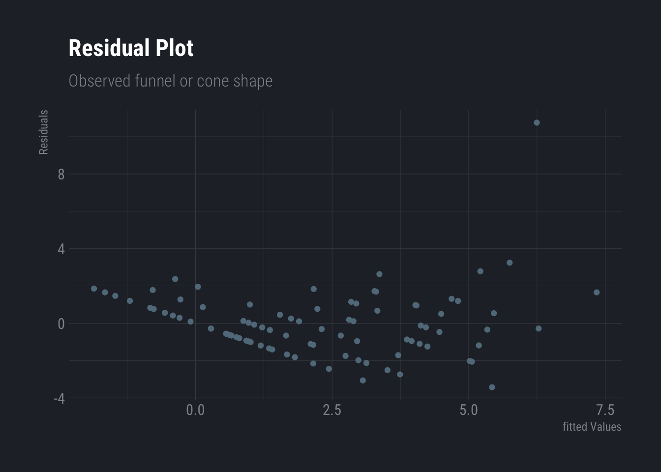
Non-linearity of the data can be checked using residue plot.
dtlm <- lm(Murder_pa_p1M ~ percent_unemployed+percent_below5k, data=dt)
ggplot(dtlm, aes(x = .fitted, y = .resid)) +
  geom_point()+
    labs(
    title ="Residual Plot",
        y="Residuals",
    x="fitted Values"
  ) +
  theme_ft_rc()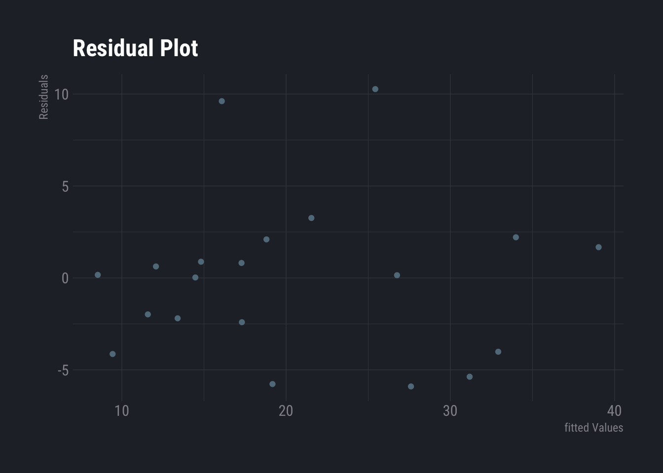
No distinct pattern is observed here. Hence, the data seems to be linear. Let us use another example to check how does non-linear one looks like.
dtlm <- lm(weight~., data=ChickWeight)
ggplot(dtlm, aes(x = .fitted, y = .resid)) +
  geom_point()+
    labs(
    title ="Residual Plot",
    y="Residuals",
    x="fitted Values"
  ) +
  theme_ft_rc()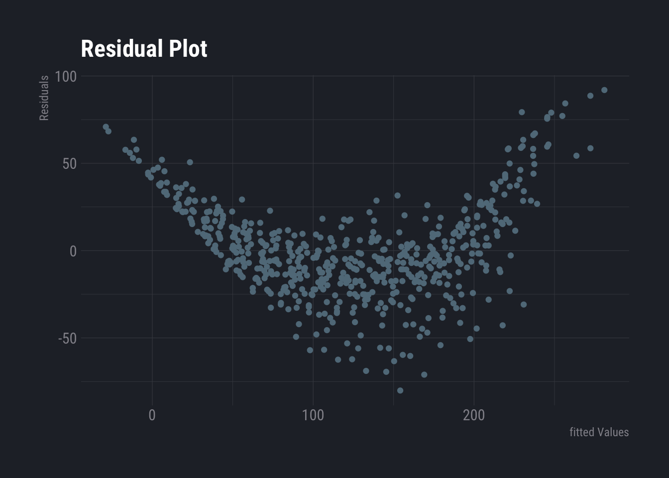
This one looks like non-linear. One needs to look for possible patterns. If a pattern is visible, it is non-linear.
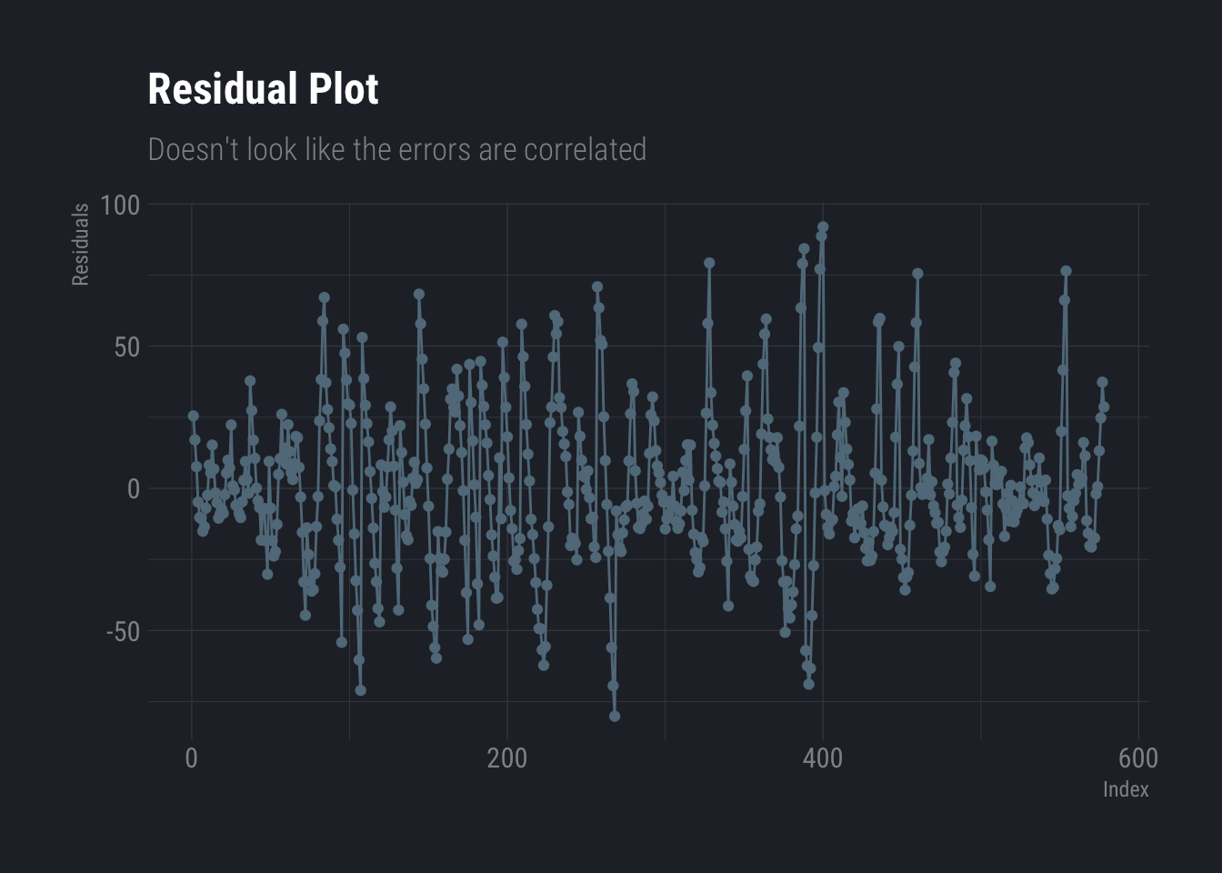
Finally, correlation of error terms is mostly observed in time series data and there are methods of cure. In non-time series data, special attention must be given to design the experiment carefully to avoid this. One can identify this graphically by plotting the residuals against the index. If no patterns are observed, i.e. you notice that the sign of the residuals change randomly, one may conclude that there is no correlation in error terms.
ggplot(data.frame(resi=dtlm$residuals, ind=as.integer(names(dtlm$residuals))), aes(x=ind,y=resi))+
  geom_line(aes(x=ind,y=resi))+
  geom_point() +
      labs(
    title ="Residual Plot",
    subtitle = "Doesn't look like the errors are correlated",
    y="Residuals",
    x="Index"
  ) +
  theme_ft_rc()