Probability Distributions

Binomial Probability Distribution

A random variable follows binomial distribution if

1. The random variable is discrete
2. The random variable is observed certain number of times (imagine tossing a coin and observing the outcome)
3. There are only two possible outcomes. One can label them as 0 or 1 or success or failure or true or false
4. There are probabilities associated with each outcome which add up to 1. If probability of success is p, probability of failure is (1-p).
5. Each outcome is independent of the other.

Probability of y successes from a random selection of n is

\[ P(y)=_nC_yp^y(1-p)^{n-y} \]

where y is the number of success, p is the probability of success and n is the sample size.

In R, one may calculate the probability using dbinom function. Suppose that you know that Messi scores 77% of the times in penalty shootout. Given this information, you want to understand that if Messi takes 5 penalty kicks, what is the probability that three of them will be goal.

dbinom(3,5,0.77)

## [1] 0.241506

What if we are asked about the probability that the number of goal will not be more than 3? There are two ways to do it. In the first way, we add up the probabilities of 0,1,2 and 3 goals.

sum(dbinom(0:3,5,0.77))

## [1] 0.3250616

In the second one, we use another function pbinom

pbinom(3,5,0.77)

## [1] 0.3250616

The mean of the distribution is sample size times the probability. In our example, we can expect 5*0.77 (3.85) goals on average out of 5 kicks. The standard deviation is \(\sqrt{np(1-p)}\).

Poisson Probability Distribution

Whenever we are dealing with number of occurrences of a particular outcome of a discrete variable in an interval, for which, average number of occurrences is known, we use Poission. For example, Number of customers arriving at a shop per day or number of goals by Messi in a month. The interval can be time, space or volume. For example, number of organisms per litre of water from a pond.

The probability of y events or observations of a particular outcome in an interval is given by

\[ P(y)=\frac{e^{-a}a^y}{y!} \] where a is the average number of events or observations of a particular outcome in an interval.

Similar to the functions in binomial, there are functions for Poisson in R as well.

Assuming that Messi scores 2 goals in every 1 matches on average, we want to calculate the probability that we will observe 2 goals in next 1 match?

dpois(1,2)

## [1] 0.2706706

If we want to know the probability of observing at least one goal, there are two ways. We can add up the probabilities of 0 and 1 goal or use ppois function.

sum(dpois(0:1,2))

## [1] 0.4060058

ppois(1,2)

## [1] 0.4060058

The mean of the distribution equals a which is already known. The standard deviation is \(\sqrt{a}\)

Normal probability distribution

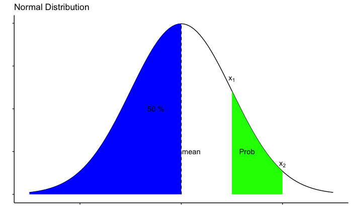
Normal probability distributions have

1. Bell shaped curve
2. Symmetrical about mean, which is the central values
3. Tails which never touch x axis (asymptotic)
4. Distribution can be described by two parameters, mean and standard deviation
5. Total area under curve is 1 and
6. probability of an interval is the area under curve of the interval range

library(ggplot2)
ggplot(data.frame(x = c(-3, 3)), aes(x)) +
  stat_function(fun = dnorm) + 
  stat_function(fun = dnorm, 
                xlim = c(-3,0),
                geom = "area",
                fill="blue") +
    stat_function(fun = dnorm, 
                xlim = c(1,2),
                geom = "area",
                fill="green")+
  labs(
    title = "(Standard)Normal Distribution",
    x="",
    y=""
  ) +
  geom_segment(x=0, xend=0, y=0, yend=0.4, linetype="dashed") +
  annotate("text", x=1, y=0.27, label=expression(x[1]))+
  annotate("text", x=2, y=0.07, label=expression(x[2]))+
  annotate("text", x=1.3, y=0.1, label="Prob")+
  annotate("text", x=0.2, y=0.1, label="mean=0")+
  annotate("text", x=-0.5, y=0.2, label="50 %")+
theme_classic() +
  theme(axis.text.x = element_blank(),
        axis.text.y = element_blank()
        ) 

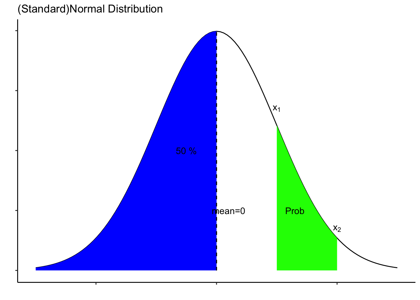
Probabilities of standard normal deviation is available in a table called z-table. Since the table provides the probabilities of standard, we convert random variable (x) to z-value.

\[ z=\frac{x-\mu}{\sigma} \] z-value basically indicates the position of the particular value of the variable in x axis (how far from mean).

In R, there is no need to use the z-table. There are functions, like in case of binomial and poisson, that can help with the calculations.

Suppose weights of students in a class has a mean of 50 and standard deviation of 5. We want to know the lower limit of top 15% weights in the class.

ggplot(data.frame(x = c(-3, 3)), aes(x)) +
  stat_function(fun = dnorm) + 
    stat_function(fun = dnorm, 
                xlim = c(2,3),
                geom = "area",
                fill="green")+
  labs(
    title = "Distribution of weights of students",
    x="",
    y=""
  ) +
  geom_segment(x=0, xend=0, y=0, yend=0.4, linetype="dashed") +
  annotate("text", x=2, y=0.07, label="lower limit")+
  annotate("text", x=0.2, y=0.1, label="mean=50")+
theme_classic() +
  theme(axis.text.x = element_blank(),
        axis.text.y = element_blank()
        ) 

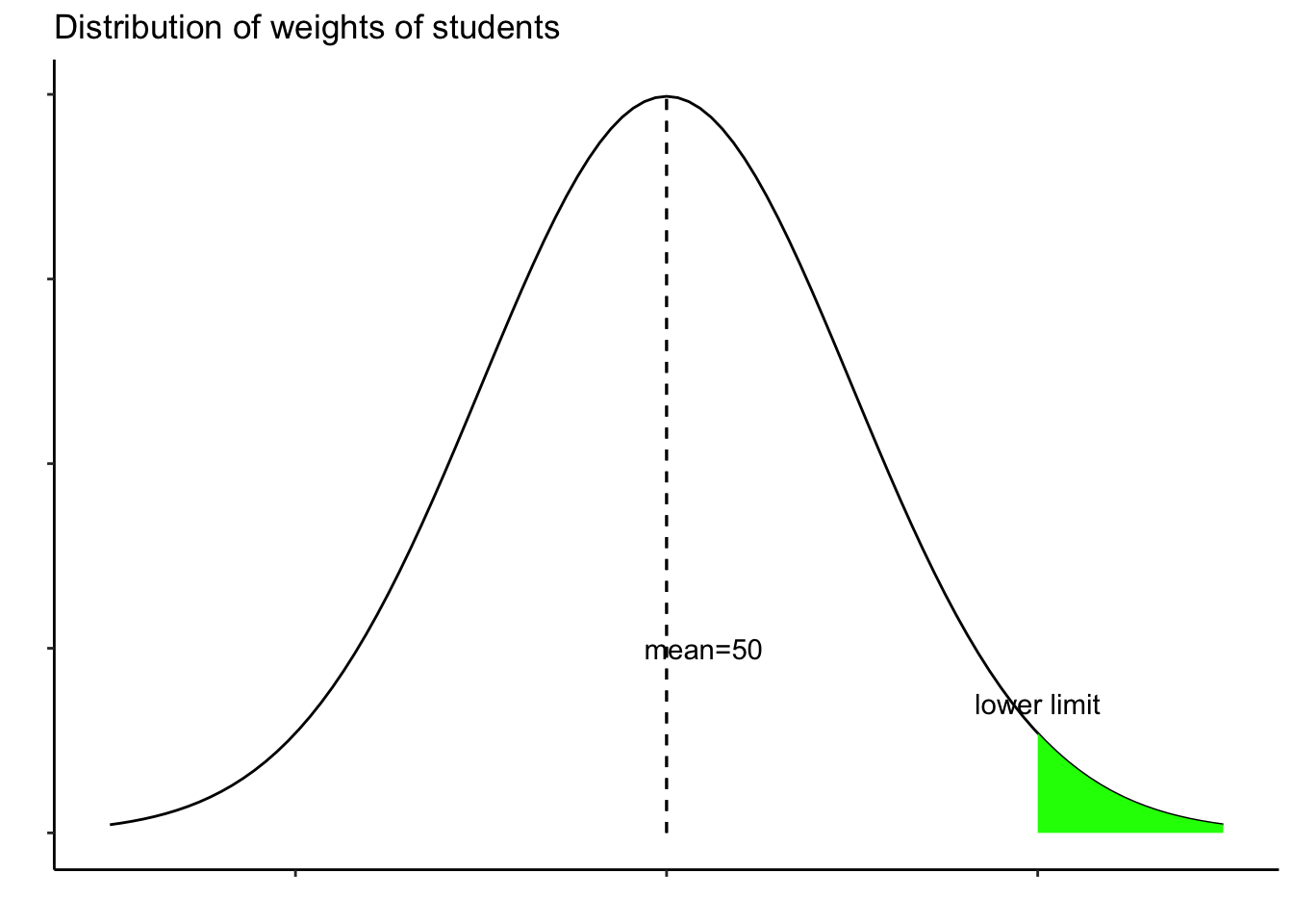
We are interested in finding the lower limit, which is 85 % (1- 15 %). So, we are interested in finding the value at this point. We can use the function qnorm to do so.

qnorm(0.85, 50, 5)

## [1] 55.18217

Two related videos are as follows.